Introduction

Within the cell, the localization of a given protein is determined by its biological function. Subcellular proteomics is the method to study protein sub-cellular localization in a systematic manner. There are two complementary ways to analysis localized proteins:

• On one hand biochemical sub-cellular fractionation experiments allow empirical quantification of protein across sub-cellular and sub-organellar compartments. Proteins are allocated to a given subcellular niche if the detected intensity is higher than a threshold. We can say that this type of data has high signal-to-noise ratio, but is available in limited amounts (primary data).

• On the other hand, databases such as GO contain large amount of information about sub-cellular proteins localisation, but this is information is blended for a many biological systems. We can say that this type of data has high low signal-to-noise, but is available in large amounts (auxiliary data).

So we want to know how to optimally combine primary and auxiliary data.💹

To do so, we need to weight both types of data. If we imagine a multivariate distribution (like a Dirichlet distribution) were all the components take values between (0,1) and all values sum up to one, we can imagine that a weight of 1 indicates that the final annotation rely exclusively on the experimental data and ignore completely the auxiliary data and a weight of 0 represents the opposite situation, where the primary data is ignored and only the auxiliary data is considered.

We could use a transfer learning algorithm to efficiently complement the primary data with auxiliary data without compromising the integrity of the former. This is implemented in the pRoloc package and it was published by Breckels et al and expanded by Crook et al using a Bayesian approach. In this post I will step-by-step walk through KNN transfer learning.

Getting the data

We start with HEK293T2011 proteomics data available in the pRolocdata package.

data(HEK293T2011)

The class of (HEK293T2011) isMSnSet instance, an efficient and established to store and handle MS data and metainformation efficiently. I am not going to discuss much about this class of objects since the field is moving towards other types of data storage such as SummarizedExperiment objects

We can also get an overview experimental data and query how many proteins across how many conditions were quantified.

head(exprs(HEK293T2011),2)

##             X113      X114       X115      X116      X117       X118       X119
## O00767 0.1360547 0.1495961 0.10623931 0.1465050 0.2773137 0.14294025 0.03796970
## P51648 0.1914456 0.2052463 0.05661169 0.1651138 0.2366302 0.09964387 0.01803788
##               X121
## O00767 0.003381233
## P51648 0.027270640

dim(exprs(HEK293T2011))

## [1] 1371    8

What is important to know is that 1371 proteins were quantified across eight iTRAQ 8-plex labelled fractions ( one could know a bit more about the experiment with ?HEK293T2011)

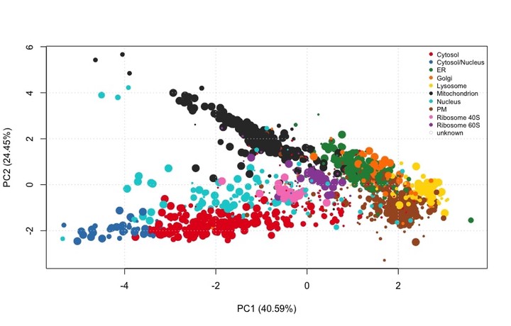
Next thing we can do is see how well these organelles have been resolved in the experiment using a PCA plot

plot2D(HEK293T2011)
addLegend(HEK293T2011, where = "topright", cex = 0.6)

Figure 1: PCA plot of HEK293T2011 subcellular proteomics dataset

We see that some organelles such as cytosol and cytosol/nucleus are well resolved - and so they will get a high weigh- while others such as the Golgi or the ER are less so - so they will get a low weight. There are some proteins that do not get annotation because the resolution of the experiment did not allow so.

Quetting auxiliary annotation (Biomart Query)

Next thing we can do is get auxiliary data. We can do so by querying biomaRt and storing the annotation as an AnnotationParams object. Again, this is part of the pRoloc package, and it has been created for efficient data handling.

ap <- setAnnotationParams(inputs =
                              c("Human genes",
                                "UniProtKB/Swiss-Prot ID"))

## Connecting to Biomart...

We can access this instance with

getAnnotationParams()

## Object of class "AnnotationParams"
##  Using the 'ENSEMBL_MART_ENSEMBL' BioMart database
##  Using the 'hsapiens_gene_ensembl' dataset
##  Using 'uniprotswissprot' as filter
##  Created on Tue Jan 26 15:47:22 2021

We can annotate our innitial HEK293T2011 data by creating a new MSnSet instance populated with a GO term as a binary matrix (so the auxiliary data with information about 889 cellular compartment GO terms has been added).

HEK293T2011goset  <- makeGoSet(HEK293T2011)

Nearest neighbour transfer learning

gtools::permutations(length(seq(0, 1, 0.5)), 3, seq(0, 1, 0.5), repeats.allowed = TRUE) 

##       [,1] [,2] [,3]
##  [1,]  0.0  0.0  0.0
##  [2,]  0.0  0.0  0.5
##  [3,]  0.0  0.0  1.0
##  [4,]  0.0  0.5  0.0
##  [5,]  0.0  0.5  0.5
##  [6,]  0.0  0.5  1.0
##  [7,]  0.0  1.0  0.0
##  [8,]  0.0  1.0  0.5
##  [9,]  0.0  1.0  1.0
## [10,]  0.5  0.0  0.0
## [11,]  0.5  0.0  0.5
## [12,]  0.5  0.0  1.0
## [13,]  0.5  0.5  0.0
## [14,]  0.5  0.5  0.5
## [15,]  0.5  0.5  1.0
## [16,]  0.5  1.0  0.0
## [17,]  0.5  1.0  0.5
## [18,]  0.5  1.0  1.0
## [19,]  1.0  0.0  0.0
## [20,]  1.0  0.0  0.5
## [21,]  1.0  0.0  1.0
## [22,]  1.0  0.5  0.0
## [23,]  1.0  0.5  0.5
## [24,]  1.0  0.5  1.0
## [25,]  1.0  1.0  0.0
## [26,]  1.0  1.0  0.5
## [27,]  1.0  1.0  1.0

th <- gtools::permutations(length(seq(0, 1, length.out = 4)), 10, seq(0, 1, length.out = 4), repeats.allowed = TRUE)

## marker classes for HEK293T2011
m <- unique(fData(HEK293T2011)$markers.tl)
m <- m[m != "unknown"]
th <- thetas(length(m), length.out=4)

Optimizing weigth

We can do a grid search to determine which is the best th, with the knntlOptimisation function of the pRoloc package.

topt <- knntlOptimisation(HEK293T2011, HEK293T2011goset,
                          th = th,
                          k = c(3, 3),
                          fcol = "markers.tl",
                          times = 50, 
                          method = "Breckels" )

For the sake of time, we can reduce our initial data, as it will take a long time to do this grid search (even if knntlOptimisation uses parallelisation by default).

set.seed(2021)
i <- sample(nrow(th), 50)
topt <- knntlOptimisation(HEK293T2011, HEK293T2011goset,
                          th = th[i, ],
                          k = c(3, 3),
                          fcol = "markers.tl",
                          times = 5)

The optimisation is performed on the labelled marker examples only. topt result stores all the result from the optimisation step, and in particular the observed theta weights, which can be directly plotted as shown on the bubble plot.

plot(topt)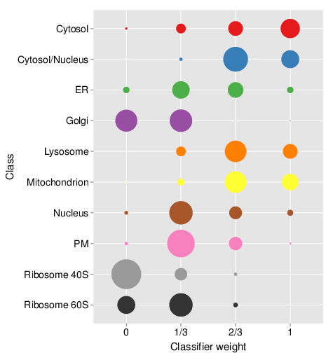

Result stocores for the optimisation step. Note that this figure is the result using extensive optimisation on the whole HEK293T2011 dataset and auxiliary HEK293T2011goset dataset, not only with only a random subset of 50 candidate weights.

We see that the cytosol and cytosol/nucleus and ER are predominantly scored with high heights, consistent with high reliability of the primary data. Golgi, PM and the 40S ribosomal clusters are scored with smaller scores, indicating a substantial benefit of the auxiliary data.

The best grid search parameters can be accessed with:

getParams(topt)

Note that the data HEK293T2011 gets annotated with the best parameters at the knntlOptimisation step. We can get the best weights with:

bw <- experimentData(HEK293T2011)@other$knntl$thetas

HEK293T2011 <- knntlClassification(HEK293T2011, HEK293T2011goset,
                                bestTheta = bw,
                                k = c(3, 3),
                                fcol = "markers.tl")

HEK293T2011 <- getPredictions(HEK293T2011, fcol = "knntl")

Plotting the results

# These functions allow to get/set the colours/points to plot organelle features 
setStockcol(paste0(getStockcol(), "80"))
#this defines the point size
ptsze <- exp(fData(HEK293T2011)$knntl.scores) - 1
plot2D(HEK293T2011, fcol = "knntl", cex = ptsze)
setStockcol(NULL)
addLegend(HEK293T2011, where = "topright",
          fcol = "markers.tl",
          bty = "n", cex = .7)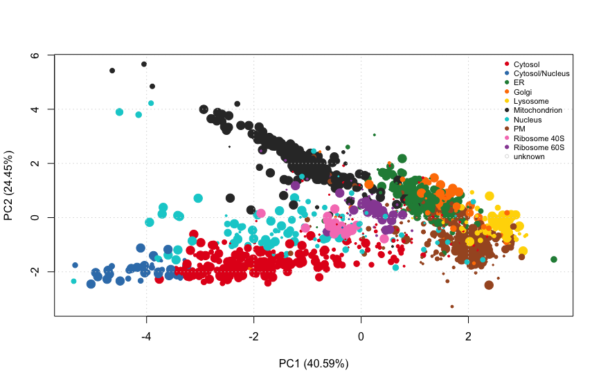

PCA plot of HEK293T2011 after transfer learning classification. The size of the points is proportional to the classification scores.

Conclusions

A weighted k-nearest neighbour transfer learning algorithm can be very useful to predict of protein sub-cellular localisation using quantitative proteomics data as primary data source and Gene Ontology-derived binary data as auxiliary data source.