Word network of Bioconductor packages
Exploration of the connections between Bioconductor packages
 Word network in Bioconductor packages titles
library(BiocPkgTools)
library(tidyverse)
library(tidytext)
library(widyr)
library(igraph)
library(ggraph)
library(lubridate)
library(emo)
Motivation
Bioconductor has a total of 5796 at the present day 2021-01-31. Therefore, navigating across Bioconductor packages can be a daunting experience. Luckily, BiocPkgTools offers a rich ecosystem of metadata around Bioconductor packages 📜.
Statistics of Bioconductor downloads
We can get a tidy data.frame with download stats for all packages using the function biocDownloadStats.
#  Getting a tidy tibble summarizing monthly download statistics
bio_download_stats <- biocDownloadStats()
bio_download_stats %>%
head(13)## # A tibble: 13 x 7
## Package Year Month Nb_of_distinct_IPs Nb_of_downloads repo Date
## <chr> <int> <chr> <int> <int> <chr> <date>
## 1 ABarray 2021 Jan 54 114 Software 2021-01-01
## 2 ABarray 2021 Feb 0 0 Software 2021-02-01
## 3 ABarray 2021 Mar 0 0 Software 2021-03-01
## 4 ABarray 2021 Apr 0 0 Software 2021-04-01
## 5 ABarray 2021 May 0 0 Software 2021-05-01
## 6 ABarray 2021 Jun 0 0 Software 2021-06-01
## 7 ABarray 2021 Jul 0 0 Software 2021-07-01
## 8 ABarray 2021 Aug 0 0 Software 2021-08-01
## 9 ABarray 2021 Sep 0 0 Software 2021-09-01
## 10 ABarray 2021 Oct 0 0 Software 2021-10-01
## 11 ABarray 2021 Nov 0 0 Software 2021-11-01
## 12 ABarray 2021 Dec 0 0 Software 2021-12-01
## 13 ABarray 2021 all 54 114 Software NAAs we see observations for all the months of the year are generated once that the year starts (download values for events in the future are filled up with 0). Also note that there is a summary statistic for month called all embedded inside the tibble, and the Date value for that observation is NA (this would makes group by date very convenient).
This tibble contains information about packages that expands from 2009 to 2021. There are 3 categories of packages, with the total number of package per category as follows:
bio_download_stats %>%
  distinct(Package, repo) %>%
  count(repo) %>%
knitr::kable()| repo | n |
|---|---|
| AnnotationData | 2659 |
| ExperimentData | 821 |
| Software | 2316 |
Full details of Bioconductor packages
The complete information for the packages as described in the DESCRIPTION file can be obtained with biocPkgList.
bpi = biocPkgList()
colnames(bpi)
## [1] "Package" "Version" "Depends"
## [4] "Suggests" "License" "MD5sum"
## [7] "NeedsCompilation" "Title" "Description"
## [10] "biocViews" "Author" "Maintainer"
## [13] "git_url" "git_branch" "git_last_commit"
## [16] "git_last_commit_date" "Date/Publication" "source.ver"
## [19] "win.binary.ver" "mac.binary.ver" "vignettes"
## [22] "vignetteTitles" "hasREADME" "hasNEWS"
## [25] "hasINSTALL" "hasLICENSE" "Rfiles"
## [28] "dependencyCount" "Imports" "Enhances"
## [31] "dependsOnMe" "VignetteBuilder" "suggestsMe"
## [34] "LinkingTo" "Archs" "URL"
## [37] "SystemRequirements" "BugReports" "importsMe"
## [40] "Video" "linksToMe" "OS_type"
## [43] "PackageStatus" "License_restricts_use" "License_is_FOSS"
## [46] "organism"There is lots of information in here. We could use this metadata information to understand the connections between packages.
Word network of Bioconductor packages
The most informative variables about the packages are Title and Description so we can explore the connections between packages doing some text mining using a Tidytext approach.
To prepare our dataset we need to initially tokenize the text. The Wikipedia definition for tokenization on lexical analysis is as follows:
Tokenization is the process of demarcating and possibly classifying sections of a string of input characters
The sections can be words, sentence, ngram or chapter (for example if analysis a book). In this case we are gonna break down package Titles or Description into words using the function unnest_tokens.
In addition, we can remove stop words (included in the Tidytext dataset).
bpi_title <- bpi %>%
  dplyr::select(Package, Title) %>%
  unnest_tokens(word, Title) %>%
  anti_join(stop_words)

bpi_description <- bpi %>%
  dplyr::select(Package, Description) %>%
  unnest_tokens(word, Description) %>%
  anti_join(stop_words)
Note that the number of words from Title is 11932 and the number of words from Description is 59370, so package Descriptions contain on average 5 times the words of package Titles.
We can have a look at how the tokenised titles for each package look like:
bpi_title## # A tibble: 11,932 x 2
## Package word
## <chr> <chr>
## 1 a4 automated
## 2 a4 affymetrix
## 3 a4 array
## 4 a4 analysis
## 5 a4 umbrella
## 6 a4 package
## 7 a4Base automated
## 8 a4Base affymetrix
## 9 a4Base array
## 10 a4Base analysis
## # … with 11,922 more rowsThem, we can use pairwise_count from the widyr package to count how many times each pair of words occurs together in the package Title. This function works as a mutate in that it takes the variables to compare and returns a tibble with the pairwise columns and an extra column called n containing the number of words co-occurrences. I think this function is very sweet 🍯!
bpi_titlepairs <- bpi_title %>%
pairwise_count(Package, word, sort = TRUE, upper = FALSE)

bpi_desciptionpairs <- bpi_description %>%
pairwise_count(Package, word, sort = TRUE, upper = FALSE)
This data is ready for visualization of network of co-occurring words in package Titles. We can use the ggraph package for visualizing this network. We are going to represent just the top co-occurring words, or otherwise we get a very populated network which is impossible to read.
set.seed(1234)
bpi_titlepairs %>%
filter(n >= 6) %>%
graph_from_data_frame() %>%
ggraph(layout = "fr") +
geom_edge_link(aes(edge_alpha = n, edge_width = n), edge_colour = "purple") +
geom_node_point(size = 5) +
geom_node_text(aes(label = name), repel = TRUE,
point.padding = unit(0.2, "lines")) +
theme_void()+
theme(legend.position="none")+
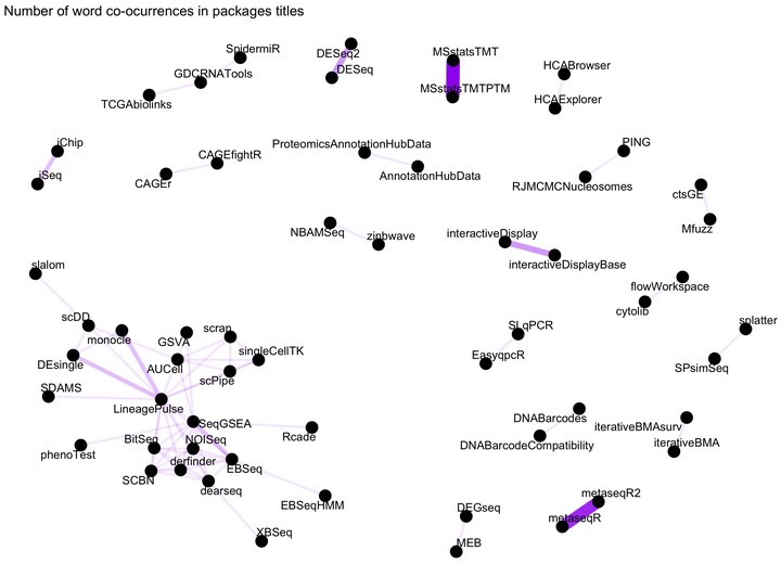
labs(title = " Number of word co-ocurrences in packages titles")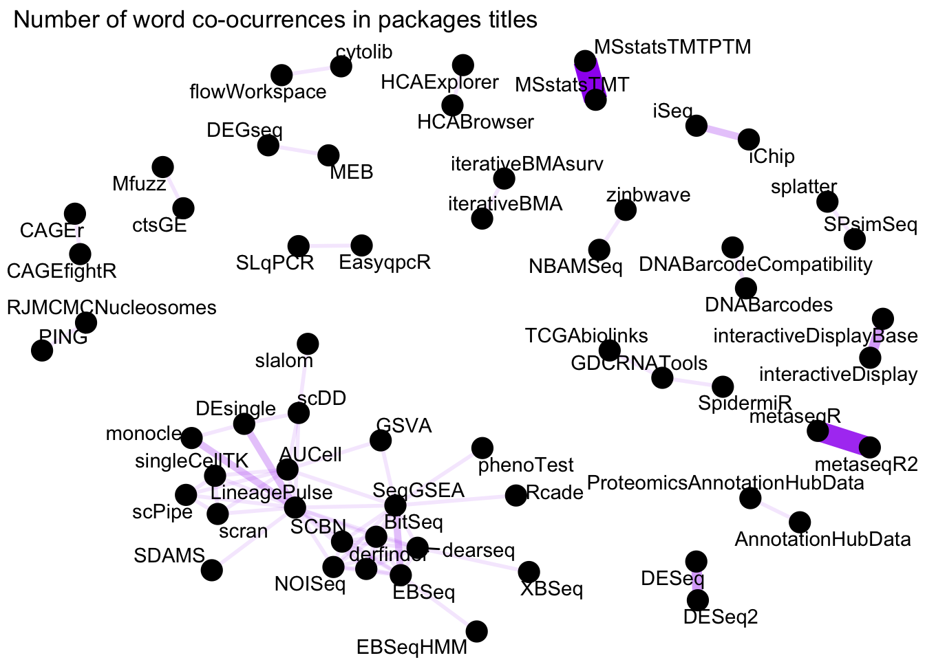
Figure 1: Word network in Bioconductor packages Titles
We see some clear and logical clustering of packages in this network.For example, DESEq and DESeq2 packages cluster together, as one would expect since they DESeq2 is the successor of DESeq. There are other obvious connections such as MSstatsTMTPTM and MSstatsTMTP since the former has added functionality to analyse PTMs on TMT shotgun mass spectrometry-based proteomic experiments. There is a big cluster on the bottom left corner with packages to analyse RNASeq and single cell RNASeq.
What about the network build from words of the Description?
set.seed(1234)
bpi_desciptionpairs %>%
  filter(n >= 15) %>%
  graph_from_data_frame() %>%
  ggraph(layout = "fr") +
  geom_edge_link(aes(edge_alpha = n, edge_width = n), edge_colour = "orange") +
  geom_node_point(size = 5) +
  geom_node_text(aes(label = name), repel = TRUE,
                 point.padding = unit(0.2, "lines")) +
  theme_void()+
  theme(legend.position="none")+
  labs(title = "Number of word co-ocurrences in packages Description")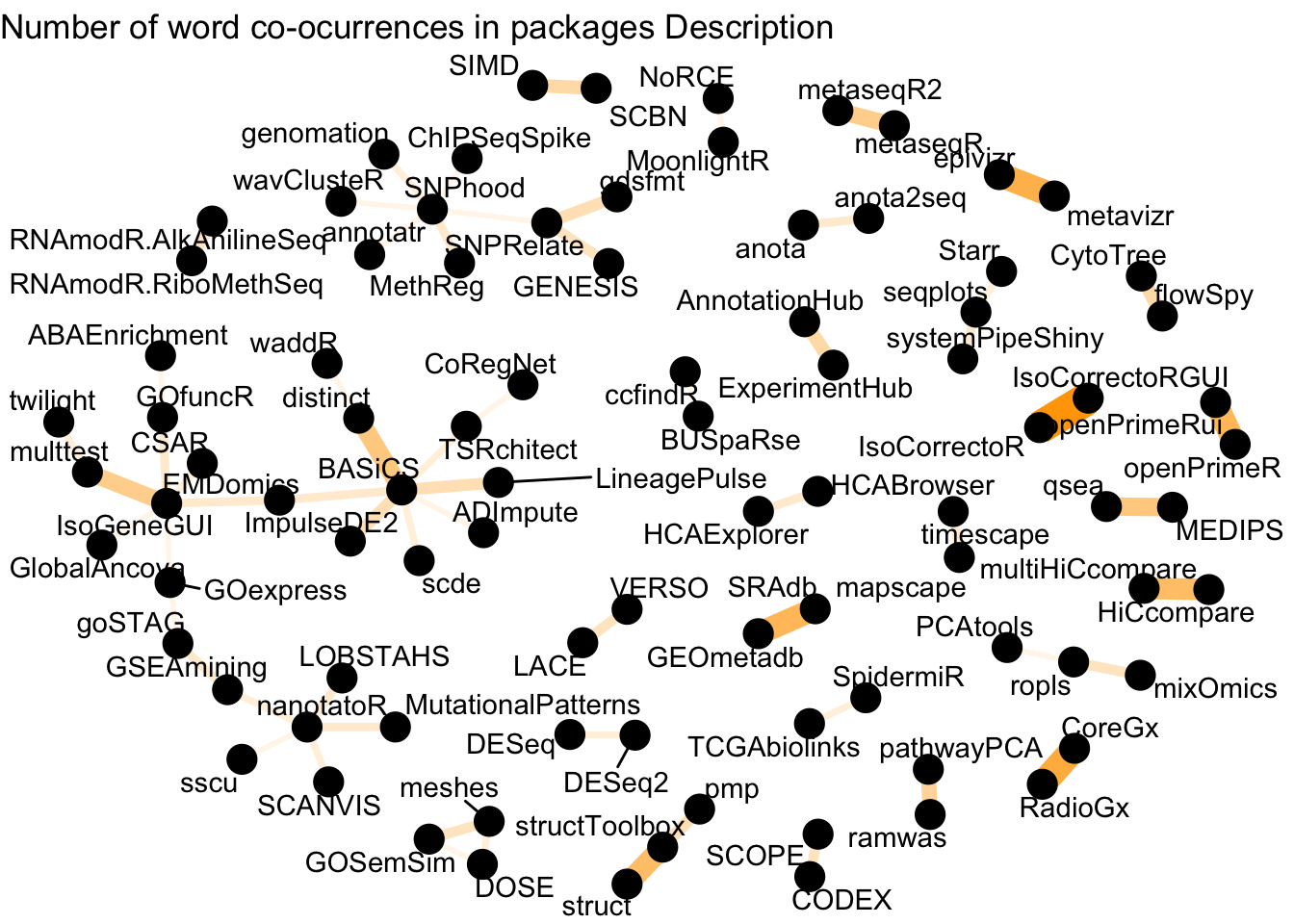
Figure 2: Word network in Bioconductor packages Description
We see more connections here, and some of the relationships are still obvious (e.g HiCcompare and multiHiCcompare, anota and anota2seq, AnnotationHub and ExperimentHub). This network is richer, and one would have to dive a bit deeper to get a better sense of this network.
Conclusions
Text mining of Bioconductor packages metadata is a straight forward visual way to understand the relationships between packages. One could go beyond this and for example finding words that are especially important across package Descriptions by calculating tf-idf statistic. One could also set up a GitHub Action executed as a CRON job to get updates periodically. This could turn into a challenge for BiocChallenges. This post was inspired by Chapter 8 of the Tidytext book and BiocRoulette.
Maria Dermit
Postdoctoral Research Scientist
Postdoctoral researcher interested in translation control and data science for biomedical research.